Overview
A classifier that learns one group of objects at a time has to do two jobs. It must keep recognizing the old categories and extract features useful for the new ones. Its final accuracy combines both jobs with the behavior of the last decision layer. Moontae and his colleagues ask what becomes visible when the encoder and classifier are tested separately.
Key Findings
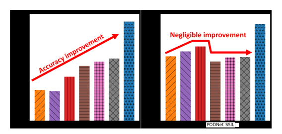
If two students sit the same test and one has a better answer sheet, the score alone says little about which one understood the material. In continual learning there is a similar ambiguity. A system can gain points because its output layer is better calibrated to old and new classes, even if the underlying representation has improved very little.
Look behind the final decision
A class-incremental model receives labeled images in stages. At test time it predicts among the categories learned so far, without being told which stage the image belongs to. An encoder turns the image into a feature vector, and an output layer turns that vector into a category decision. A good final accuracy can come from better features, better decisions given the same features, or a mix of both.
The paper freezes each trained encoder and tries other ways of classifying its features. A linear probe learns a new linear decision layer. A nearest-neighbor probe asks whether images close together in the learned feature space share labels. The authors also examine transfer to other datasets and compare how similar representations are across stages. Figure 2 shows what each measurement holds fixed.
The rankings change when the classifier changes
These rows are from Table 1 for the 10-task ImageNet-100 experiment.
| Method | Final accuracy (%) | Frozen-encoder linear probe (%) | Frozen-encoder nearest neighbors (%) |
|---|---|---|---|
| Joint training | 75.56 | 74.28 | 69.62 |
| Fine-tuning | 37.20 | 56.08 | 52.04 |
| BiC | 44.60 | 61.58 | 56.36 |
| PODNet | 50.70 | 53.42 | 40.26 |
| AFC | 54.90 | 55.68 | 49.33 |
AFC has a substantially higher final accuracy than fine-tuning in this setting, while fine-tuning roughly matches AFC on the linear probe and clearly exceeds it on the nearest-neighbor probe. BiC also improves both probes over fine-tuning. The paper finds that SSIL’s learned classifier closely resembles a freshly trained linear probe. PODNet and AFC use specialized cosine classifiers, providing another way for final accuracy to improve. In the 11-task setting, which starts with a larger base task, the feature rankings change again. The paper also shows that aligning first-stage feature quality can narrow later differences between methods.
Try the features somewhere else
The experiments also use frozen encoders for classification on resized CIFAR-10, STL-10, and CUB-200 bird images. BiC reaches 52.20 in the 10-task out-of-domain evaluation, ahead of AFC at 46.39. In the 11-task setup, which begins with more classes, AFC reaches 58.38 and BiC 51.71. Comparing the representations across stages with centered kernel alignment gives another view of how features change over time. Figures 5–6 · Table 1 This puts pressure on an explanation based solely on rebalancing the old classifier. A change that truly makes features more informative should have a chance to help a fresh head or a related task. The numbers from frozen encoders show why both comparisons matter. Fine-tuning performs poorly with its own final classifier yet yields features that a new classifier can use.
Where the standard ranking comes apart
The experiments examine regularization-based continual learning methods. A system can become better at preserving the old classifier’s output, while the features it passes to that classifier become less separable. Looking at the classification and representation tests together makes that distinction visible. The work gives benchmark designers a way to ask which part of an apparent advance actually traveled with the encoder.
Questions & Answers
The opening answers are simulated author responses based on the paper.
Q: Why freeze the encoder for a probe?
A: Freezing it keeps the learned features fixed. Training a fresh classifier then asks how useful those features are when the original decision layer is removed from the comparison.
Q: Does this make the usual accuracy score less useful?
A: It remains the direct measure of whether the current system recognizes the accumulated categories. The extra measurements answer whether the features may be useful under another classifier or another task.
Q: Why does the first stage matter?
A: A first-stage model trained on more classes or for more epochs can give later updates a stronger starting representation. Comparing algorithms with different first-stage models can then attribute some of that starting advantage to later updates. Our alignment experiments help expose that dependence.
Q: Can one transfer score settle which encoder is best?
A: A probe measures what a particular readout can learn from frozen features, with its given labels and training budget. A linear probe, nearest-neighbor readout, and a downstream adaptation can therefore order the same encoders differently. The benchmark is clearest when the starting model is fixed and the report includes both end-to-end accuracy and probes aligned with the intended transfer.
Future Ideas
Give visual model updates a transfer audit
For a collection whose image labels evolve over time, record the same encoder checkpoints for each update strategy. Keep an untouched set of image categories and a distinct image collection for small transfer tests. Before releasing an update, compare its ordinary classification score with the performance of fixed-budget probes trained on the held-out tasks.
Compare a release rule based on accuracy alone with one that also requires retained transfer utility. Evaluate both over several sequences of category arrivals. Measure downstream labeling effort, old-category regressions, and how often the transfer check flags a model that looked better on the main benchmark.
Preregister the transfer tasks and probe budgets. Repeat the comparisons across seeds and report paired uncertainty for the differences, especially if a release decision hinges on a small gain.
Sources
Original abstract
Class incremental learning (CIL) algorithms aim to continually learn new object classes from incrementally arriving data while not forgetting past learned classes. The common evaluation protocol for CIL algorithms is to measure the average test accuracy across all classes learned so far -- however, we argue that solely focusing on maximizing the test accuracy may not necessarily lead to developing a CIL algorithm that also continually learns and updates the representations, which may be transferred to the downstream tasks. To that end, we experimentally analyze neural network models trained by CIL algorithms using various evaluation protocols in representation learning and propose new analysis methods. Our experiments show that most state-of-the-art algorithms prioritize high stability and do not significantly change the learned representation, and sometimes even learn a representation of lower quality than a naive baseline. However, we observe that these algorithms can still achieve high test accuracy because they enable a model to learn a classifier that closely resembles an estimated linear classifier trained for linear probing. Furthermore, the base model learned in the first task, which involves single-task learning, exhibits varying levels of representation quality across different algorithms, and this variance impacts the final performance of CIL algorithms. Therefore, we suggest that the representation-level evaluation should be considered as an additional recipe for more diverse evaluation for CIL algorithms.