Overview
A scientific archive contains words like “neuron,” “layer,” and “signal” in many kinds of papers. A narrower term can reveal what a topic is really about, but adding thousands of terms makes a conventional word-pair matrix grow quickly. This paper changes how that matrix is approximated so a topic model can use more of the vocabulary.
Key Findings
Why a topic about neurons needs the word "kanji"
Picture a topic model reading an archive of NeurIPS papers. One topic leads with "layer," "recognition," "hidden," "word" and "speech." That list could describe almost any neural network paper. Moontae asks how a model can see the specific vocabulary behind such a topic, and what it costs to keep thousands of rare terms in play.
The quadratic wall around spectral topic models
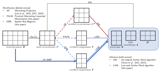
The authors build on Joint-Stochastic Matrix Factorization. A word-document matrix counts how often each of vocabulary words appears in each of documents. From it, the method forms a word co-occurrence matrix , which records how often pairs of words appear together. Equation 1 gives the following unbiased estimate.
Here is the count vector of document , is its length, and the diagonal term removes each word's pairing with itself. The Anchor Word algorithm then splits into topics and topic correlations, assuming each topic has an anchor word that appears only in that topic.
Real data breaks the model's assumptions. The empirical is often indefinite and full rank, and rare words make greedy anchor selection pick outliers. The authors' earlier Alternating Projection step repairs so it is normalized, non-negative and positive semi-definite with rank equal to the number of topics . That repair costs quadratic time and memory, because the non-negativity projection turns a sparse matrix dense. The authors report that this limits spectral inference to small vocabularies.
Rectifying while compressing
The first new method, Epsilon Non-Negative rectification (ENN), starts from the observation that the non-negativity projection changes only a few entries. Its output is nearly a rank- matrix plus a sparse correction. ENN stores only and the sparse correction, and it finds the entries needing correction by checking the rows of with the largest norms. A Cauchy-Schwarz bound shows that other entries cannot fall far below zero. Matrix-vector products then cost time.
The second method, Proximal Alternating Linearized Minimization rectification (PALM), minimizes a direct fit with forced non-negative:
This is Equation (2). The authors prove the gradients are Lipschitz continuous (Lemma 1), which supports global convergence and an adaptive step size. PALM still needs the full .
Finding anchors without the big matrix
The Low-rank Anchor Word algorithm (LAW) works directly from . Lemma 2 shows that column-pivoted QR on the full matrix picks the same anchors as the same procedure on a small -column factor, because an orthogonal embedding preserves lengths. The least-squares step that assigns every word to topics shrinks the same way. Cost falls from to . The authors say LAW is exact when and robust in practice when it has small negative entries.
The full Low-Rank Joint Stochastic Matrix Factorization pipeline (LR-JSMF) skips altogether. It applies to vectors through , uses a one-pass randomized eigendecomposition to initialize ENN, then runs LAW. The authors note a limit. When is large and the eigenvalue gap is small, a few extra power iterations make it multi-pass.
Matching the old pipeline, far faster
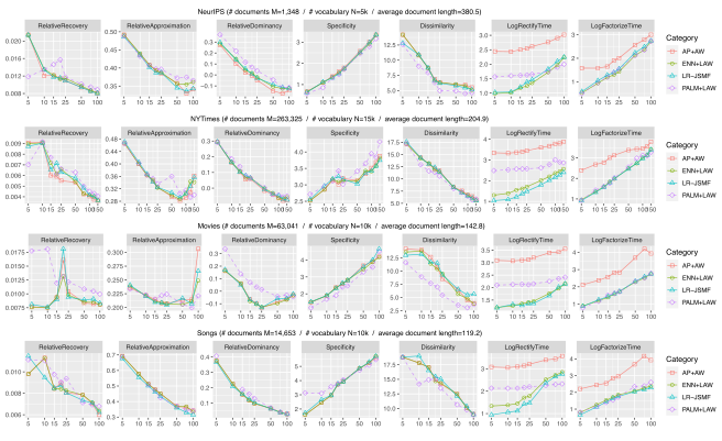
The authors tested on NeurIPS, New York Times, Movielens ratings (Movies) and Yes.com playlists (Songs). Metrics include relative approximation error, topic correlation, specificity and dissimilarity. In Figure 3, ENN+LAW and LR-JSMF track AP+AW with no visible accuracy loss, run one to two orders of magnitude faster, and LR-JSMF shows very low variance across runs. PALM deviates slightly while following the trend. Figure 2 shows ENN and LR-JSMF recovering the same anchor convex hulls as AP, while PALM differs but beats the unrectified baseline.
Reading the anchor's neighbors
Anchor words are often too rare to interpret. The authors therefore define characteristic words as the terms that co-occur most with the anchor, and read them beside the usual prominent words. Table 1 uses 10,000 NeurIPS words. A topic with prominent words "neuron, cell, circuit" gains "biological" among its characteristic words, which marks it as neuroscience. The speech topic gains "character, kanji, radical," which points to written language recognition.
| Prominent words (from B) | Characteristic words (from C) |
|---|---|
| neuron cell circuit synaptic layer signal | neuron synaptic potential cell biological circuit |
| layer recognition hidden word speech net | character samples kanji recognition radical layer |
| control action dynamic optimal policy reinforcement | tpdp control states optimal action dynamic |
What happens as the vocabulary grows
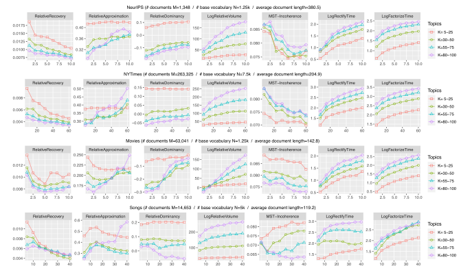
For the second experiment the authors picked the top words by tf-idf, with LR-JSMF only, since full matrices no longer fit. As rises, anchor hulls grow relative to random hulls, relative recovery error falls, and the paper's minimum-spanning-tree incoherence measure generally falls, while runtimes stay stable. The authors read this as better anchors and better separability from larger vocabularies. They report that vocabularies above 15k do not fit in memory with earlier algorithms. They omit specificity and dissimilarity here, since distances over different supports can't be compared.
Questions & Answers
Q: Why keep a rare anchor if readers may not recognize it?
A: The anchor serves a mathematical role in estimation. The paper shows characteristic neighbors so a reader can interpret the signal it contributes without relying on the rare word alone.
Q: Does more vocabulary always mean better topics?
A: The experiments show benefits across the reported settings. Adding very noisy or irrelevant terms can create new problems. Vocabulary selection and the size of the compressed representation remain modeling decisions.
Q: What does the compressed method preserve?
A: It approximates the co-occurrence structure needed to estimate topics and their pairwise relationships. It does not aim to reproduce every empirical word-pair count exactly.
Q: Was compressed inference compared with dense inference at the largest vocabulary sizes?
A: The matching result concerns anchor selection under the stated factorization conditions. At the largest scales, the dense alternatives did not fit and the comparison is among compressed versions. Smaller cases let the researchers compare pipelines directly. For a new corpus, memory and topic quality still need to be measured as compression rank and vocabulary change.
Future Ideas
Let a curator inspect the specialist words behind a theme
Build an archive browser for a large technical collection. For each theme show common topic words, characteristic anchor neighbors, and a few supporting documents. Include a comparison view that shows whether the theme persists when the vocabulary or approximation rank changes.
Compare it with a browser that shows prominent words alone. Ask blinded curators to distinguish close themes and retrieve niche documents. Measure interpretation accuracy, labeling time, and stability on a held-out time period, along with the memory and compute needed to regenerate the map.
Record the vocabulary-selection rule and run a small grid over topic count and compression rank. Reviewing the same curated themes across that grid shows whether a memory saving also changes which associations readers can recognize.
Sources
Original abstract
Across many data domains, co-occurrence statis- tics about the joint appearance of objects are powerfully informative. By transforming unsu- pervised learning problems into decompositions of co-occurrence statistics, spectral algorithms provide transparent and efficient algorithms for posterior inference such as latent topic analysis and community detection. As object vocabularies grow, however, it becomes rapidly more expensive to store and run inference algorithms on co-occur- rence statistics. Rectifying co-occurrence, the key process to uphold model assumptions, becomes increasingly more vital in the presence of rare terms, but current techniques cannot scale to large vocabularies. We propose novel methods that si- multaneously compress and rectify co-occurrence statistics, scaling gracefully with the size of vo- cabulary and the dimension of latent space. We also present new algorithms learning latent vari- ables from the compressed statistics, and verify that our methods perform comparably to previous approaches on both textual and non-textual data.