Overview
A geolocation model can use fine-grained classes to distinguish streets and neighborhoods. Every extra subdivision, though, leaves another candidate to score at prediction time. Moontae and his team use branch-and-bound to make that search selective. They organize classes in a tree, estimate how promising each branch could be, and skip branches whose best possible result would cost too much.
Key Findings
Give the classifier a tree it can search
Section 1 starts with the familiar Bayesian decision. To choose a class for input , maximize its likelihood times its prior:
Instead of holding the candidate classes in a flat list, the chapter arranges them hierarchically. An internal node summarizes a group of training examples by their means, variances, and coordinate ranges. Each branch carries the fraction of its parent’s examples assigned to that child. Multiplying those fractions along a route gives the prior probability of reaching a leaf.
For the probabilistic model, each subclass uses a Gaussian for each feature and assumes the features are independent given the subclass. The authors describe fitting a tree by repeatedly estimating two subclasses and assigning each training example to the more likely one. A single split is coarse, and repeated splits create finer subclasses. The chapter also describes how hierarchical k-means could support the same idea with distance as the score.
A branch can rule itself out
If a query coordinate falls outside a node’s range, its distance to the nearest edge is a lower bound on its distance to any descendant mean inside that range. A coordinate inside the range contributes zero to this bound. A separate bound can account for the smallest remaining path cost.
The authors also examine a bound using standardized deviations. They illustrate why assuming that every child’s standard deviation decreases is risky. Their parent set has sample standard deviation 4.16333. Depending on the split, one or both of the children can have a higher deviation.
| Child 1 | Child 2 | Standard deviation, child 1 | Standard deviation, child 2 |
|---|---|---|---|
| {−5, −1} | {1, 5} | 2.82843 | 2.82843 |
| {−5, 1} | {−1, 5} | 4.24264 | 4.24264 |
| {−5, 5} | {−1, 1} | 7.07107 | 1.41421 |
The chapter considers whether tree building could make its combined deviation term decrease from parent to child. It presents that property as a conjecture.
Use a cost threshold to limit each search pass
The search expressed in Equation 4 pays an edge cost when it descends from node to child . A leaf pays its fit cost . The best remaining cost satisfies
The chapter uses iterative-deepening A* (IDA*). Each pass searches depth-first and stops descending whenever the cost already paid plus a lower bound on what remains exceeds the current threshold. If the pass yields no solution within that threshold, it raises the threshold and repeats. This revisits some states but keeps memory use linear in search depth. The usual guarantee of finding the same optimum as exhaustive search depends on the bound never overstating the cheapest completion.
Compare how many nodes the two searches visit
To test trees with up to 60 billion mixture components, the authors generate each node on demand from deterministic seeds. The same parent index reproduces the same child probabilities and subdivisions. This lets both algorithms traverse the same synthetic tree without storing all its nodes.
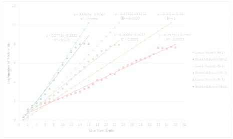
In the binary-tree tests, the chapter reports nearly two orders of magnitude fewer node visits. Its conclusion estimates that a comparable visit budget could reach roughly 1.37 times as deep with branch-and-bound. The experiment measures visits on synthetic trees. A real-world latency comparison would also account for the work needed to compute a bound at each node.
Questions & Answers
Q: When can the search safely discard a branch?
A: The lower bound must be no higher than the cheapest attainable cost among the branch’s leaves. If the cost already paid plus that lower bound exceeds the current threshold, no completion in that branch can fit within the threshold.
Q: Do Equations 1 and 2 give exactly the same likelihood score?
A: The printed Equation 2 omits the factor on the squared term that follows from taking the negative log of Equation 1. The chapter does not say whether the equation or the Gaussian likelihood was used in the experiment implementation. A reproduction should specify the objective and check its pruned predictions against exhaustive search under that same objective.
Q: Where would this help most?
A: A tree whose node statistics give tight bounds can eliminate many candidates near the root. If the feature ranges overlap heavily, a query may fall inside many bounding boxes and the search will have to inspect more of them. The chapter identifies Reuters RCV1 and Gene Ontology as proposed real-data tests for that question.
Future Ideas
For a product catalogue, train a hierarchy of product types and store each subtree’s range of observed feature values. Compare the original distance bound with a bound that also uses the observed range of descendant variances. First prove that the tighter bound remains valid for the chosen leaf score. Then compare labels against exhaustive scoring and measure both visits and latency on frequent and rare categories.
Sources
Original abstract
In a typical machine learning classification task there are two phases: training and prediction. This paper focuses on improving the efficiency of the prediction phase. When the number of classes is low, linear search among the classes is an efficient way to find the most likely class. However, when the number of classes is high, linear search is inefficient. For example, some applications such as geolocation or time-based classification might require millions of subclasses to fit the data. Specifically, this paper describes a branch-and-bound method to search for the most likely class where the training examples can be partitioned into thousands of subclasses. To get some idea of the performance of branch-and-bound classification, we generated a synthetic set of random trees comprising billions of classes and evaluated branch-and-bound classification. Our results show that branch-and-bound classification is effective when the number of classes is large. Specifically, branch-and-bound improves search efficiency logarithmically.