Overview
An archive of articles has many ways to group related words. Some are intuitive, like business or courts. Others begin with a term that appears in a short burst and rarely returns. This paper studies why an anchor-based topic model can prefer those unusual terms, and how a compact map can make its choices easier to inspect.
Key Findings
Why a topic called "cavalry" went wrong
Imagine reading the first twelve topic anchors a model picked from 41,000 New York Times articles from 2007. The greedy method from earlier anchor-word work offered cavalry, biodiesel, h/w, kingsley and mourners. Each word names a topic, yet few readers would call any of them the center of a newspaper's coverage. Moontae starts from this puzzle. He asks why a provably efficient algorithm keeps choosing such odd words, and whether a picture could show the reason.
The anchor words algorithm of Arora and colleagues assumes every topic has an anchor word that occurs with non-negligible probability only in that topic. It represents each vocabulary word by its co-occurrence pattern with every other word, then picks K anchors (K is the user's chosen topic count) and rebuilds all other words as convex combinations of the anchors' patterns. The greedy search picks the farthest point from the current selection at each step. Moontae argues that early picks tend to be infrequent, idiosyncratic words with short, intense bursts of co-occurrence. The authors report that this also yields many near-duplicate topics. In a 2008 political blog corpus, 37 of 100 greedy topics had obama, mccain, bush, iraq or palin as the top word, including 17 for obama, and only 66% of topics had a unique top word.
Why a rare word makes a vague topic
The authors explain the damage with Bayes' rule. Few words relate to cavalry, so the probability of the topic given a word barely changes across words. The topic's word distribution then collapses toward the corpus-wide distribution:
Here is a word, is a topic, and is the overall word frequency. A topic shaped like the whole corpus says little, and several such topics look alike.
Drawing the hull instead of guessing it
The paper reverses the earlier recipe. Earlier work found an approximate hull around exact high-dimensional vectors, with each word reduced to roughly 1,000 random dimensions. Moontae computes the exact convex hull of an approximate set of vectors, by projecting the co-occurrence matrix to two or three dimensions with t-SNE or PCA. They use the Quickhull algorithm, and the hull's vertices become the anchors. In the 3D setting the input is 0.03% as wide as the original New York Times matrix.
t-SNE turns distances between words into pair probabilities, then places points in low dimensions so the two probability sets match by minimizing the Kullback–Leibler divergence, a measure of mismatch between distributions. In the paper's Equations 1–4, the high-dimensional similarity uses a Gaussian kernel and the low-dimensional similarity uses a heavy-tailed one. The objective is
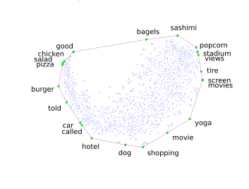
Figure 1 shows the 2D version for Yelp reviews. The authors present 2D maps only as illustrations and report that 3D works better in practice. The projection also sets topic count. In their figures a 2D hull has 21 vertices and a 3D hull has 69, so users tune granularity by changing the embedding dimension. The cost is an upper limit on topics for a given projection. In the experiments, t-SNE chose 69, 77 and 107 anchors for Yelp, blogs and the Times, and PCA chose 49, 32 and 47. Figure 2 shows PCA bunching words together, which the authors blame for its lower anchor counts.
What the new anchors look like
The datasets are Yelp (20,000 documents, 1,606 word types), political blogs (13,000, 4,447) and the Times (41,000, 10,713), from Table 1. Table 2 lists the first anchors each method chose for the Times corpus.
| Rank | t-SNE | PCA | Greedy |
|---|---|---|---|
| 1 | police | beloved | cavalry |
| 2 | bonds | york | biodiesel |
| 3 | business | family | h/w |
| 11 | court | board | yiddish |
Table 3 pairs five randomly chosen t-SNE topics with the closest topic from each other method. It reports each anchor's hard rank, its zero-based position in its own topic's word list. In the Times topics, the t-SNE anchors police and senator both have hard rank zero. The greedy anchor for the matching police topic has hard rank 198. The authors note that t-SNE and PCA often agree, which suggests linear and non-linear projections both find more relevant anchors.
Measuring topics beyond coherence
The authors define several metrics for the three-dimensional embeddings. Recovery error (Equation 5) averages the residual left when each word is rebuilt from the anchors. Normalized entropy (Equation 6) measures how evenly a word spreads across topics. Topic specificity (Equation 7) is the average KL divergence between each topic and the corpus distribution. Topic dissimilarity (Equation 8) measures how far each topic sits from the average topic.
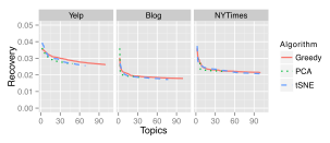
Figure 4 shows recovery error is similar across methods. t-SNE is slightly better than greedy. Entropy is lower for t-SNE and PCA, and both show higher specificity and dissimilarity at small topic counts. The greedy topics sit closer to the corpus and to each other.
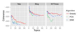
Coherence, which rewards top words that share documents, favors greedy. The authors explain that frequent corpus words often appear together, so many corpus-like topics earn high coherence while having low specificity. They ask readers to read it alongside the other metrics.
Saliency, held-out likelihood and stability
Soft rank (Equation 10) averages the log ratio between a topic's top word probability and its anchor's probability, with lower values meaning a more prominent anchor. The authors report that t-SNE anchors stay relatively more probable as topics increase, while greedy anchors become more prominent only gradually.
Held-out probability required a fix. Early t-SNE runs scored badly because anchor words, which are frequent, had probability set to zero in other topics and produced large negative log values. The authors added 10⁻⁵ to those zero entries for all models and renormalized. After that, t-SNE beat greedy, most clearly on the Times. They note the greedy method on the unprojected matrix beat t-SNE on Yelp but does not scale. They also stress this metric is sensitive to smoothing.
Because t-SNE is stochastic, the authors ran five initializations per dataset. Anchor counts varied from 59 to 69 on Yelp (43 shared by at least four runs), 80 to 95 on blogs (56 shared), and 83 to 107 on the Times (51 shared). Anchor sets are therefore only partly stable. They reserve a 5% holdout to measure document likelihood. In separate synthetic experiments, none of the methods reliably recovers the planted anchors, so the paper concentrates on what the algorithms find in real corpora.
Questions & Answers
Q: Is a visible anchor a label for the whole topic?
A: It is a starting point for estimating the topic’s word distribution. Readers can examine the associated words and representative documents before giving the topic a name.
Q: Why try three dimensions?
A: A higher-dimensional projection can expose more hull vertices. The paper’s Yelp examples have 21 in two dimensions and 69 in three. More vertices give a user finer-grained candidates, although some can still be hard to interpret.
Q: Can the map hide a topic?
A: Any compact embedding discards information. A topic that is distinct in the full space may no longer occupy an exposed position. That makes comparisons with other projections and selected document samples useful.
Q: Would the same anchor words appear if we drew the map again?
A: The embedding is stochastic. Different seeds can expose different words as hull vertices, so a single map gives one candidate set. Inspecting anchors alongside representative documents and topic-word rankings makes them easier to evaluate, while repeating the projection measures whether a theme depends on one drawing.
Future Ideas
Give a public archive a map of its topic choices
Build a browsing interface for a collection of public meeting notes. Show anchor words on a projected map and link each one to the documents and nearby words that helped form it. Let a curator test a second projection when a useful group appears missing.
Compare projected and greedy anchors in a blinded study with the same vocabulary and number of topics. Ask curators to find documents related to named issues, label topic groups, and explain why they made their choices. Track rare topics separately and report how often the map leads to a mistaken grouping.
Repeat the blinded curator test across several embedding seeds at matched topic counts. Show the distribution of results and record which anchor words recur, since consistent analyst performance and consistent anchor identity are different outcomes.
Sources
Original abstract
The anchor words algorithm performs provably efficient topic model inference by finding an approximate convex hull in a high-dimensional word co-occurrence space. However, the existing greedy al- gorithm often selects poor anchor words, reducing topic quality and interpretability. Rather than finding an approximate con- vex hull in a high-dimensional space, we propose to find an exact convex hull in a visualizable 2- or 3-dimensional space. Such low-dimensional embeddings both improve topics and clearly show users why the algorithm selects certain words.