Overview
A full attention layer lets every token compare itself with every other token. That makes it expressive and increasingly expensive as the sequence grows. SBM-Transformer takes a different route. Each head first decides which token pairs to keep by sampling from a learned graph model, then computes attention along those sampled connections.
Key Findings
A sequence where every token must meet every other
Picture the paper's synthetic puzzle. A model reads 256 integers and must label each position 1 if its value appears elsewhere in the sequence, and 0 otherwise. With a single attention head and 32 hidden dimensions, the head must compare every token with every other token to reach perfect accuracy. Many efficient Transformers that shortcut attention lose here. Moontae and his colleagues built SBM-Transformer so a head can start sparse and still grow to full attention when a task demands it.
Sampling a graph instead of scoring every pair
Full attention scores every query–key pair, which costs time and memory that grow with the square of sequence length. The authors keep the masked variant of attention, where a binary matrix switches pairs on or off and only the active scores enter the softmax (their Equations 3 and 4). Most sparse Transformers fix or hash this mask. Here each head samples it fresh for every input.
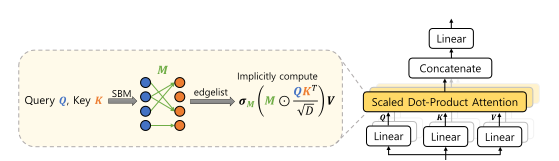
A stochastic block model generates a random graph from latent clusters. Each node holds a membership weight for each of clusters, and a small block matrix says how likely clusters are to link. The authors use a mixed-membership version. A head passes queries and keys through a two-layer network, compares them with trainable cluster embeddings , and obtains soft memberships and . The block matrix comes from comparing the clusters with each other (Equations 5 to 8). Then:
Here is the chance that query attends to key . The authors sample with the fastRG algorithm of Rohe and colleagues, which draws a Poisson-distributed number of edges and places each one directly. Cost therefore follows the number of edges, which the input itself influences, and the full score matrix never appears. Figure 3 of the paper shows how node and cluster positions yield dense, block-diagonal or very sparse masks.
Teaching a sampler with a straight-through gradient
Drawing edges is a discrete step, so ordinary backpropagation stops there. The authors use a straight-through estimator. For each sampled edge, the gradient with respect to its probability is
where is the masked score matrix (Equation 9). The loss can therefore raise or lower the probability of every edge that was sampled. Unsampled edges get no signal, so the authors add a small perturbation to each probability during training, which lets a collapsed edge be revived.
A natural worry is that the model would always favor full attention. The authors offer a reasoned explanation rather than a proof. Dense attention is limited by head dimension and softmax, and masking adds another way to shape attention. Their LRA models settle at roughly 20% to 30% density without any penalty.
Proving the sparse model has not lost expressive power
The authors prove that SBM-Transformer approximates any continuous sequence-to-sequence function in expectation (Theorems 1 and 2). They build on conditions that earlier work established for sparse Transformers. Three block models supply a within-cluster pattern and two relay patterns that link every pair of tokens, with expected edges. Two caveats apply. The proof adds self-loops by hand, and the authors found that dropping them works slightly better in practice (59.40 versus 59.93 average LRA accuracy). The result also covers the expected output over sampled masks.
Learning to use full attention
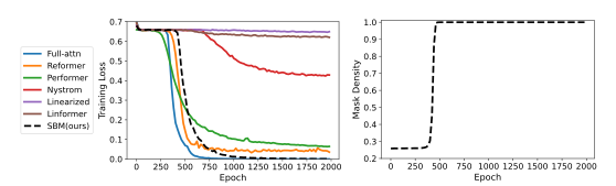
In the repeated-token task of Figure 4, full attention converges quickly and the Linear Transformer, Linformer, Reformer, Performer and Nyströmformer fail to reach perfect accuracy. SBM-Transformer with 128 clusters converges more slowly and reaches zero loss while its mask density climbs.
Long Range Arena, a penalty, and the bill for sparsity
In the Long Range Arena benchmark (five tasks, two layers and two heads per model), SBM-Transformer averaged 59.93% accuracy against 59.27% for full attention and 59.41% for Nyströmformer (Table 1). It beat full attention on all five tasks while sampling roughly 18% to 29% of possible edges. Reformer fell to 22.92% on ListOps, which the authors attribute to block-diagonal masks handling hierarchy poorly.
Adding a penalty weight on mask density cuts edges further (Table 2, accuracy with density in parentheses).
| Retrieval | Pathfinder | Average accuracy | |
|---|---|---|---|
| 0 | 80.00 (29.46%) | 75.12 (18.56%) | 59.93 |
| 79.93 (24.62%) | 75.46 (5.16%) | 60.00 | |
| 80.44 (6.99%) | 72.79 (3.76%) | 59.84 | |
| 79.46 (2.49%) | 73.79 (2.61%) | 59.37 |
At , Table 3 reports FLOP counts of 0.07 to 0.29 times full attention. Relative peak memory ranges from 0.19 to 1.01, with Text the one task that does not save memory. Density also varies with the input. On Pathfinder, the authors saw under 5% density for visually simple images and much denser attention for harder ones, and they present this as a conjecture. The two layers of the same model diverge by more than 10% on ListOps and Image.
On four GLUE tasks with a small BERT, SBM-Transformer scored 89.8 on SST-2 (tied with full attention) and 85.2 on QQP (highest), then 83.5 on MNLI and 83.6 on QNLI. Fine-tuned masks averaged 13.5% density. This model also uses a 64-token sliding window, which the authors found helpful.
The authors also acknowledge a practical limit. Unstructured sparse operations are poorly optimized on GPUs, so runtimes can exceed dense attention even when arithmetic and memory drop.
Questions & Answers
Q: What happens if a token pair is left out?
A: The head does not compute that pair’s attention score for the sampled graph. Information can still travel through other connections, heads, or layers. Whether the network recovers a particular relationship depends on the learned pattern and task.
Q: How can the model learn from a random edge draw?
A: The forward pass uses a discrete mask. During training, the straight-through estimator passes a gradient signal to the probabilities used to sample it. That provides a practical update rule without making the graph draw differentiable.
Q: Does retaining 5.16% of attention edges imply a 19-fold speedup?
A: That percentage describes the mask on Pathfinder in one configuration. The rest of the model still runs, the graph has to be sampled, and sparse kernels can be inefficient. The right performance comparison measures elapsed time and memory directly.
Q: Does the expressivity theorem cover the exact sparse model used in the main benchmarks?
A: The guarantee is in expectation for a construction that includes each token’s self-edge. The authors omit that restriction in the main experiments after observing slightly lower accuracy with it. The theorem shows that the sparse construction can express the desired operation under its conditions. Actual masks, distant evidence, and hardware costs are assessed separately.
Future Ideas
Route attention around the evidence in a long technical report
The paper adds a local sliding window for its GLUE language experiments. Start with that combination and measure longer inputs separately.
Train a document model with adaptive masks on long reports in which annotators identify the passages needed to answer a question. Give it an initial edge budget, then let it increase density on reports with evidence spread across sections. A first version could run on a fixed GPU and escalate difficult documents to a dense model.
Compare it with an optimized dense baseline and a fixed sparse baseline at the same memory limit. Measure answer accuracy, evidence recall across section boundaries, and tail latency. Deliberately place rare but decisive facts far apart to test whether the adaptive mask saves work on easy reports while preserving distant links when they are needed.
Sources
- NeurIPS 2022 paper record
- arXiv paper, including Figures 1–3 and Tables 1–3
- Authors’ SBM-Transformer implementation
Original abstract
To overcome the quadratic cost of self-attention, recent works have proposed various sparse attention modules, most of which fall under one of two groups: 1) sparse attention under a hand-crafted patterns and 2) full attention followed by a sparse variant of softmax such as -entmax. Unfortunately, the first group lacks adaptability to data while the second still requires quadratic cost in training. In this work, we propose SBM-Transformer, a model that resolves both problems by endowing each attention head with a mixed-membership Stochastic Block Model (SBM). Then, each attention head data-adaptively samples a bipartite graph, the adjacency of which is used as an attention mask for each input. During backpropagation, a straight-through estimator is used to flow gradients beyond the discrete sampling step and adjust the probabilities of sampled edges based on the predictive loss. The forward and backward cost are thus linear to the number of edges, which each attention head can also choose flexibly based on the input. By assessing the distribution of graphs, we theoretically show that SBM-Transformer is a universal approximator for arbitrary sequence-to-sequence functions in expectation. Empirical evaluations under the LRA and GLUE benchmarks demonstrate that our model outperforms previous efficient variants as well as the original Transformer with full attention. Our implementation can be found in https://github.com/sc782/SBM-Transformer .