Overview
Readings of a process may arrive at uneven times. Some will help forecast the next hour, and others may be stale or noisy. The authors assign a neural agent to each time-stamped observation and let those agents contribute to a continuous-time forecast. A cooperative training rule helps the model decide whose information should count at different prediction times.
Key Findings
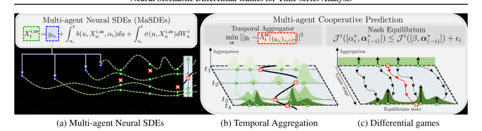
A forecast that listens to more than the latest measurement
A monitor records a brief spike in pollution, then takes its next reading much later. The spike may matter for the forecast. It might also be a bad observation. How recent it was is only one clue. The authors build a forecasting model that lets each available reading influence the future differently at different times. A measurement with a delayed effect can grow more important several steps ahead. A misleading reading can have less influence when the others offer a more coherent prediction.
Follow one path from each reading
The model assigns one neural agent to each observed timestamp. Here an agent is a learned part of the forecast. Each agent starts from its observation and uses a stochastic differential equation to carry information into the forecast interval. A differential equation describes how the predicted state changes continuously, while a random term allows a distribution of future paths. This lets the model use timestamps as they arrive, including irregularly spaced observations.
One path can tell only part of the story. The combined predictor puts time-dependent attention weights on the agents’ proposed changes. In Equation 2, is the weight on agent , is its drift term, is the diffusion covariance, and is the gradient of the log density conditioned on its reading. The gradient points toward locally more probable states. The weights sum to one, so assigning more influence to one agent means less influence for others.
Figure 1 traces the separate trajectories, their weighted prediction, and the training game.
A game that rewards cooperation
The training objective uses the error of the combined forecast and a terminal cost on each individual trajectory. The authors frame the interaction as a cooperative stochastic game. An agent can reduce its influence when other agents help the shared prediction more. Solving the agents’ coupled optimization problems together becomes difficult as the number of observations grows. The training method uses fictitious play. It holds other agents’ actions from the preceding round fixed while learning an individual response. The paper connects this procedure to an approximate Nash equilibrium under stated assumptions. Its noise analysis also gives a conditional bound on forecast error in which the weight assigned to a perturbed reading matters. This is a mathematical argument for the method’s design alongside the empirical tests.
When a measurement from farther back matters more
The synthetic experiment uses the Mackey–Glass delay equation. The current state depends on a state at a fixed interval in the past. That creates a case where it matters which earlier measurements the predictor listens to. The proposed method’s MSE was 0.055 in Table 2, compared with 0.074 for CRU and 0.128 for Neural Laplace. In the qualitative plot, the weights show how the model draws on the region around earlier, informative states. See the attention weights and prediction in Figure 2.
How the forecast handles a noisy reading
In the real-data tests, each forecast uses the first 80% of a sequence to predict the final 20%. Table 1 reports the following mean squared errors, in units of , for air quality, speech, and Physionet observations.
| Method | Beijing air quality | Speech Commands | Physionet |
|---|---|---|---|
| Neural Laplace | 0.3633 | 0.4547 | 0.5550 |
| CRU | 0.3613 | 0.4464 | 0.5081 |
| CSDE-TP | 0.3481 | 0.4460 | 0.3958 |
| Proposed model | 0.2892 | 0.4087 | 0.3829 |
In the separate air-quality stress test, the authors draw perturbation times from a Poisson process and inject Gaussian noise during evaluation. The model’s MSE rises from 0.314 to 0.340 as the reported noise setting rises from 0.1 to 1.0. CRU goes from 0.370 to 0.448, and CSDE-TP from 0.359 to 0.849. This is evidence about the injected noise used in that experiment. It leaves questions about sensor drift or outages, and about the cost of running a model whose number of agents grows with the number of observations. See Table 3 and Figure 3 for the perturbation test and sample paths.
Questions & Answers
Q: Why use a continuous-time model?
A: It allows the predictor to work with the observation timestamps directly and describe a forecast between them. That is useful when measurements arrive at irregular intervals.
Q: Why do the components need to cooperate?
A: Each component only represents one piece of the history. Training them toward a shared forecast allows the model to reduce the influence of an observation when other observations are more informative.
Q: Does the noise result cover every sensor failure?
A: The paper tests a defined noise model on the air-quality data. Other failures, such as calibration drift or a whole sensor going offline, call for separate evaluation.
Q: Can the white-noise experiment tell us how expensive the model is as observations accumulate?
A: The experiment tests robustness to a specified perturbation. With one agent per past observation, a longer history also adds computational work. The paper reports no direct runtime or memory comparison. A controlled deployment comparison would hold forecast intervals and solver budgets fixed while varying the number of observations.
Future Ideas
Forecast through a known equipment fault
Build a retrospective test from equipment sensor streams with maintenance logs and independent fault annotations. Compare the cooperative predictor with a similarly sized continuous-time attention model. Evaluate the same forecast windows before, during, and after failures involving drift, gaps, and sudden spikes.
Measure error by forecast horizon and the frequency of confident failures under each fault type. Inspect whether changes in learned observation weights correspond to the logged faults. The forecast should be judged on held-out equipment and compared at the same inference cost before it guides any real intervention.
Keep the lookback duration fixed and record runtime and memory by the number of available observations inside it. Irregularly sampled streams can differ in this count even when they cover the same time window.
Sources
Original abstract
Modeling spatiotemporal dynamics with neural differential equations has become a major line of research that opens new ways to handle various real-world scenarios (e.g., missing observations, irregular times, etc.). Despite such progress, most existing methods still face challenges in providing a general framework for analyzing time series. To tackle this, we adopt stochastic differential games to suggest a new philosophy of utilizing interact- ing collective intelligence in time series analysis. For the implementation, we develop the novel gra- dient descent-based algorithm called deep neural fictitious play to approximate the Nash equilib- rium. We theoretically analyze the convergence result of the proposed algorithm and discuss the advantage of cooperative games in handling non- informative observation. Throughout the exper- iments on various datasets, we demonstrate the superiority of our framework over all the tested benchmarks in modeling time-series prediction by capitalizing on the advantages of applying cooper- ative games. An ablation study shows that neural agents of the proposed framework learn intrinsic temporal relevance to make accurate time-series predictions.