Overview
A topic model can find words about control systems and words about neural circuits. It can also ask whether those topics tend to occur together. That second answer should behave like a probability. Earlier spectral methods could infer negative entries from real corpora. Moontae traces the problem to a mismatch between empirical word counts and the mathematical structure their inference algorithms expect.
Key Findings
Five topics, and four of them say "neuron layer hidden"
Picture a topic model asked for just five topics on the NIPS conference papers. The earlier Anchor Word method of Arora and colleagues keeps returning words such as neuron, layer, hidden, and signal across its lists. Moontae starts from this failure. Spectral inference promises speed, determinism, and provable guarantees, yet on real documents it often yields unusable output and leans on ad-hoc fixes. Their paper reframes the task and explains why the failure happens.
One framework for topics, pixels, and playlists
The authors call the general problem Joint Stochastic Matrix Factorization. A matrix holds the joint probability that two objects appear together, such as two words in a document. The goal is to approximate it as
Here gives the probability of each object within each of latent clusters, and gives the joint probability of pairs of clusters. and are joint-stochastic, meaning they behave like joint distributions. is column-stochastic, meaning each column sums to one. Table 1 of the paper lists the same structure for documents, images, networks, legislatures, and playlists. Topics are the special case where objects are words.
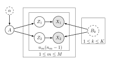
Identifiability comes from the separability assumption. Each cluster has a basis object, called an anchor word for text, that has positive probability only in that cluster. Under this assumption the factorization is unique up to reordering the clusters.
What the true matrix must look like
The authors then ask what the ideal co-occurrence matrix looks like. It equals , where averages over documents and is document 's topic distribution. For any vector , the quantity is an average of squared terms and cannot be negative. So is positive semidefinite and also entrywise nonnegative, which the authors call doubly nonnegative. The same holds for , which is also low-rank.
Empirical matrices built from limited data are generally full-rank and indefinite, with many negative eigenvalues. The paper argues that the earlier Anchor Word algorithms ignored this mismatch. The observed matrix for document uses Equation 5:
counts the objects in document , and is its length. Subtracting the diagonal count removes each object's pairing with itself. This estimator is unbiased under the paper's sampling model, yet any single sample can still stray far from the ideal structure.
Rectifying the matrix before choosing anchors
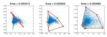
The proposed fix projects toward the ideal set before inference. The paper's preferred method, Alternating Projection, cycles through three adjustments in the style of Dykstra's algorithm. One keeps only the largest positive eigenvalues, which forces positive semidefiniteness and rank . One shifts all entries equally so they sum to one. One clips negatives to zero. The authors also describe a lighter method, Diagonal Completion, which changes only the diagonal and appears in their appendix.
The rest of the pipeline follows. A new pivoted QR routine exploits sparsity, replacing random projections and keeping inference deterministic. Probabilities for each object come from simplex-constrained quadratic programs solved with exponentiated gradient. The topic-topic matrix comes from a simple formula using the anchor submatrix and the diagonal matrix of anchor rows of :
Dividing by a diagonal matrix cannot create negative entries, and submatrices of positive semidefinite matrices stay positive semidefinite. The recovered therefore stays doubly nonnegative. The authors note that essentially this recovery appeared in earlier work but could not yield a valid topic-topic matrix without rectification.
What the topics and interactions look like
The experiment spans the two document corpora and two collections of item selections in Table 2.
| Dataset | Training examples | Vocabulary | Mean example length |
|---|---|---|---|
| NIPS | 1,348 | 5,000 | 380.5 |
| NYTimes | 269,325 | 15,000 | 204.9 |
| Movies | 63,041 | 10,000 | 142.8 |
| Songs | 14,653 | 10,000 | 119.2 |
In Table 3, on NIPS with , the baseline repeats frequent words across topics, as the opening scene showed. Alternating Projection separates a neural topic (neuron, circuit, cell, synaptic) from a control topic (control, action, dynamic, optimal, policy). The authors report that its topics resemble those from Gibbs sampling in Mallet. On Movies with , they report a cluster of Disney animation mostly from the 1990s and a cluster of fantasy films led by Lord of the Rings, while the baseline repeats Pulp Fiction and Silence of the Lambs 15 times.
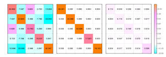
Figure 3 tests the topic-topic matrix directly. The earlier method produces large negative entries. A probabilistic reconstruction removes negatives but lacks off-diagonal structure and does not sum to one. The rectified version gives a valid joint-stochastic matrix.
Measuring across topic counts
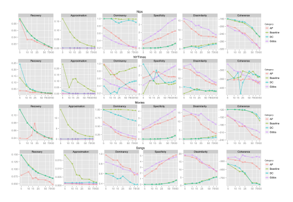
Figure 4 compares the baseline, Diagonal Completion, Alternating Projection, and Gibbs sampling on six measures across all four corpora. These cover recovery error, approximation error, diagonal dominancy, specificity, inter-topic dissimilarity, and coherence. The authors report that Alternating Projection reduces recovery error in almost all cases and beats Diagonal Completion. Its specificity, dissimilarity, and coherence track Gibbs sampling, while the baseline and Diagonal Completion repeat the corpus distribution. All metrics use the original , though and come from the rectified matrix.
Caveats appear in the paper itself. Held-out probability is left out because relative results depend on smoothing parameters. A high coherence score can coexist with repetitive topics, since the metric rewards terms that appear together. On semi-synthetic data, differences between methods are smaller, and the authors speculate that such data is more well-behaved than real text, which may explain why the problem went unnoticed.
Why rectification helps and where the proof stops
Rare words often become anchors under pivoted QR, because their sparse, noisy rows stand out. That makes the anchor submatrix highly diagonally dominant and uninformative about topic correlation. The authors argue the low-rank projection suppresses noisy rare-word rows and the positive semidefinite projection restores missing diagonal information. In Songs, the baseline's dominancy becomes undefined beyond when a chosen song occurs at most once per playlist, while Alternating Projection stays valid.
On convergence, they invoke local linear convergence results of Lewis, Luke, and Malick. Two conditions are argued, one through prox-regularity of the rank-constrained set. The third, strong regularity, is expected from noise and not verified a priori. Empirically, the ratio of average distances between iterations stayed at or below 0.9794 on NYTimes. The authors also note that the original guarantees should hold better for the rectified matrix. They leave open how anchors in the rectified space form better bases, and whether recursive application to could learn super-topics.
Questions & Answers
Q: Why care whether a matrix entry is negative?
A: A negative topic-pair probability has no direct probabilistic interpretation. It signals that the recovered factors may not describe the joint process the model assumes.
Q: Why repair the input before recovering the topic matrix?
A: The input statistics help determine the anchors and later factors. Adjusting only the final topic matrix leaves any unreliable anchor choices in place. Rectifying the input can affect both stages.
Q: Would every use of this factorization require text?
A: The framework treats word pairs as one example of observed pairs. The same representation can describe other objects with recorded co-occurrences, subject to the model assumptions and the quality of the measurements.
Q: Does a valid topic matrix establish that each relationship is real?
A: Rectification makes the matrix obey the structural requirements of the model, and the proof describes local convergence under its assumptions. In finite data, a structural correction can also change empirical counts. For a particular relationship, look for support in held-out word pairs and persistence when documents or vocabulary choices change.
Future Ideas
Track which topic associations survive new samples
Build a topic monitor for an archive of public records. Fit the rectified model on consecutive time periods and resample documents within each period. Display a topic link only when its relative strength and rank among a topic’s partners are stable across resamples and supported by held-out co-occurrences.
Compare the monitor with the original spectral method and a probabilistic topic model at similar runtime. Measure held-out pair prediction, stability of topic words, and the number of links curators can substantiate by reading documents. Use known topic shifts and deliberate vocabulary perturbations to see which links persist for the wrong reason.
Sources
Original abstract
Spectral inference provides fast algorithms and provable optimality for latent topic analysis. But for real data these algorithms require additional ad-hoc heuristics, and even then often produce unusable results. We explain this poor performance by casting the problem of topic inference in the framework of Joint Stochastic Matrix Factorization (JSMF) and showing that previous methods violate the theoretical conditions necessary for a good solution to exist. We then propose a novel rectification method that learns high quality topics and their interactions even on small, noisy data. This method achieves results comparable to probabilistic techniques in several domains while maintaining scalability and provable optimality.