Overview
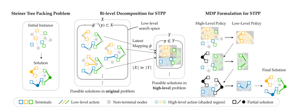
Suppose several groups of terminals must be connected over one network. Each group can find a cheap route by itself. When the groups all choose the same link, the combined plan can be impossible. The Steiner tree packing problem asks for a low-cost collection of trees that connects the terminal groups without sharing nodes or edges. HCO learns how to break up that joint decision.
Key Findings
Routing one tree uses up options for the next
A Steiner tree can use intermediate nodes to connect a group of terminals cheaply. Each tree in a packing solution must also leave the other groups enough network to reach their terminals. If is the set of edges chosen for group and is the weight of an edge, the cost to minimize is . To be feasible, each must contain a tree spanning its group, and the trees must have disjoint vertex sets.
Commit a little, then replan
The high-level policy selects a candidate region for the next set of terminals. The low-level solver uses that region to build a tree. The next high-level decision sees the resources the new tree has used. This is the essential difference between the iterative plan and allocating all regions at the start. In the two-stage method, a single division sets the regions before any tree is built. In HCO, each actual tree determines what resources remain, so a later region can still use nodes an earlier candidate region included but its tree left untouched.
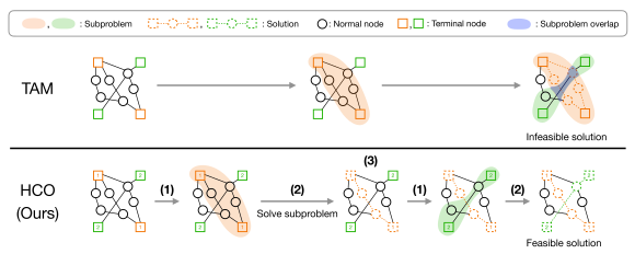
The high-level policy chooses a vertex set for group . Write for the trees that span the group's terminals inside the induced subgraph . In this notation, the low-level problem from Equation 10 is
This optimization gives the learner feedback on a proposed region. The region determines the choices the solver can see. Once it returns a tree, HCO only removes the vertices that tree used. The authors initialize the high-level policy with examples from OR-Tools and then fine-tune it with reinforcement learning. Decomposition and training, Sections 4–5
Choose what the deadline can buy
Selected Table 1 results for 80-node instances are averages over four seeds. Gap is the average relative excess in cost over the optimum among solved cases. The feasible fraction includes every test instance.
| Method | Gap ↓ | Feasible fraction ↑ | Time (ms) ↓ |
|---|---|---|---|
| HCO | 0.054 | 0.932 | 124 |
| Two-stage divide method | 0.246 | 0.620 | 47 |
| Flat learning method | 0.087 | 0.902 | 529 |
| PathFinder-SP | 0.150 | 0.976 | 20 |
| Unrestricted MILP | 0.000 | 1.000 | 1648 |
PathFinder-SP found feasible solutions more often and ran faster on this test. HCO's solutions were closer to optimal on average. At 100 nodes, the flat learning method found feasible solutions slightly more often than HCO, at 90.5% versus 89.2%. When all three learning methods trained on 40-node graphs had to solve the same 100-node cases, HCO's average gap was 0.059, compared with 0.260 for the flat policy and 2.910 for two-stage decomposition. That comparison holds the set of solved cases fixed. Tables 1–2
Inspect the choices the policy makes before routing
Some nodes are especially costly to reserve. A trap node leaves a subsequent terminal group disconnected if an earlier tree claims it. On the 40-node, two-net test, the reported likelihood of selecting a trap node fell from 0.494 for two-stage decomposition to 0.422 for HCO. Selection of redundant nodes also fell, from 0.747 to 0.608. The likelihood of selecting nodes in optimal solutions remained close, at 0.898 for two-stage decomposition and 0.887 for HCO.
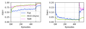
The learning curves show why the two metrics sometimes move in different directions. Once the learner solves a difficult case for the first time, that case enters the average cost gap and can raise it. The curves mark the transition from supervised training to reinforcement learning. Node selection, Table 3
Questions & Answers
The opening answers are simulated author responses based on the paper.
Q: Why can’t the trees be optimized independently?
A: Their choices interact. A route selected for one group can occupy a node or edge another group needs. The decomposition has to preserve those constraints.
Q: Does HCO certify optimality?
A: Its low-level solver handles smaller problems. The learned decomposition can constrain which global solutions are reachable, so the unrestricted solver remains the quality reference in the experiment.
Q: Why compare route costs only on graphs every method solved?
A: One method might return cheap routes because it solves only the easiest cases. Comparing costs on the common solved set gives each method the same instances. Report overall feasibility beside it to reveal how often a method leaves a graph unrouted. Generalization to larger generated graphs still depends on topology and how the terminals were selected.
Future Ideas
Retry the decomposition that blocks a critical route
For a routing simulator, log which terminal group becomes disconnected after each split. Spend a fixed wall-clock retry budget only where a cheaper independent connectivity check detects a bottleneck. Compare against HCO alone and a time-limited solver on unseen graph families. Measure feasibility, cost on common solved instances, and time at the 95th percentile.
Charge all decomposition retries and mixed-integer subproblem solves to the same wall-clock budget. In addition to larger graphs, hold out graph families with bottleneck patterns that differ from training.