Overview
A playlist can mix jazz with blues, or rock with country. A topic model that mostly rediscovers pop and rock because they dominate the collection tells a listener very little. This paper turns a fast spectral topic model into a practical pipeline and checks whether it can recover a more useful picture from noisy word or item counts.
Key Findings
Why a topic model that loves pop and rock tells a listener so little
Picture a music service that groups playlists into fifteen themes. The correlated topic model of Blei and Lafferty, run with default settings on playlists from Yes.com, produced topics that mostly mixed Pop and Rock. That mirrors the genre makeup of the whole corpus, so a playlist with only a couple of Rock songs would land in a generic Pop and Rock blend. Moontae builds on this puzzle. He asks what it takes to make spectral topic modeling, which estimates topics from word co-occurrence counts instead of repeated passes over documents, reliable enough for real data.
Counting pairs instead of rereading documents
The authors work within Joint Stochastic Matrix Factorization. A matrix records how often each pair of words appears together in a document. The method factors it as
Here holds one word distribution per topic, and holds the probability that two topics co-occur, so it captures topic correlations. One parallel pass over the corpus builds , and inference never revisits individual documents. The authors contrast this with tensor decomposition, which uses third-order statistics. In their account, the popular CP version needs uncorrelated topics and captures only weak negative correlations through a user-chosen Dirichlet prior. The alternative Tucker decomposition needs sparsity constraints and many more parameters.
Rectification and the five-step pipeline
Spectral methods break easily when real counts disagree with the model. The paper's Rectified Anchor Word algorithm runs five steps. Step 0 builds . Step 1 rectifies it by alternately projecting onto low-rank, positive semidefinite, nonnegative, and normalized matrices. Step 2 finds one anchor word per topic, a word the separability assumption says occurs only with that topic. Step 3 recovers by writing every word's row as a convex mixture of anchor rows. Step 4 recovers topic correlations as
where is the set of anchor words and is their co-occurrence block. Anchors are usually rare words, so their counts are noisy, and the authors say rectification balances those entries.
The authors contribute several implementation choices. They find that Douglas-Rachford iterations also rectify, at nearly twice the cost of alternating projection. They develop a sparse implicit pivoted QR for anchor finding that needs space and leaves untouched. For Step 3 they add an alternating direction method of multipliers solver and an exact active-set solver, as alternatives to exponentiated gradient, whose learning rate is hard to tune. They also release MATLAB and Python code.
How much rectification and pruning are enough

Figure 2 shows that five iterations often suffice and 15 to 20 match the 150 iterations of earlier work. Figure 1 examines vocabulary pruning on NeurIPS and NYTimes, varying the share of documents a word may appear in. The authors conclude that proper pruning is necessary.
Comparing against tensors, variational inference, and Gibbs sampling
The authors tested NeurIPS, NYTimes, two small text sets (Blog and Yelp) and two preference sets (Movies and Songs). They scored topics with six metrics, including specificity, dissimilarity, coherence, and sparsity, and avoided relying on held-out likelihood alone. They caution that coherence can mislead when topics duplicate frequent words, so they treat closeness to Gibbs sampling as the guide.
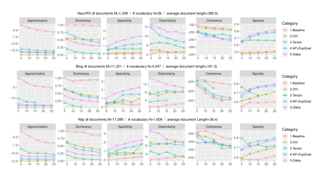
In Figure 3, tensor decomposition beats the unrectified baseline and online variational inference but behaves inconsistently as topics increase. Rectified anchor inference with exponentiated gradient tracks Gibbs most closely. In Figure 4, ADMM and active-set solvers improve specificity and sparsity over exponentiated gradient. The authors choose ADMM because it is insensitive to its settings (, ) and much faster than active-set.
On NeurIPS with five topics (Figure 6), online variational inference repeats "cell" and "neuron" across topics, and tensor decomposition spreads "neuron" and "layer" everywhere. AP+ADMM and Gibbs produce distinct themes.
Speed and the genre test
The authors report timings in Section 5 and Figure 6.
| Comparison | Reported result |
|---|---|
| Tensor, 5 topics on NeurIPS | 5 hours |
| Tensor, 25 topics on Yelp | 48 days |
| AP+ADMM on small datasets | Under a minute |
| AP+ADMM on NYTimes | Under an hour (15 AP iterations) |
| AP+ADMM vs online variational | About 4 times faster on NYTimes |
| AP+ADMM vs Gibbs | About 40 times faster on NYTimes |
| Variational CTM, 50 topics on Songs | 6 hours |
| AP+ADMM, 50 topics on Songs | Under 10 minutes |
Tensor decomposition did not finish for 20 to 25 topics on Blog, which explains two missing points in Figure 3. Online variational inference runs faster on NeurIPS, though the authors judge RAW's topic quality worth the cost.
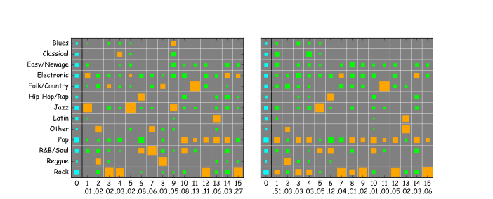
Figure 5 returns to the playlists. AP+ADMM finds three Jazz topics (Electronic, Pure, Blues) and four Rock topics (Folk Rock, Rock n Roll, Pop style, Alternative Rock). The variational model also puts high marginal probability on topic 1, the one closest to the corpus genre mix. The authors argue this can raise likelihood while producing an unhelpful classifier for new playlists.
Caveats come from the authors. Movies show weaker genre structure than Songs, because people watch recent releases, so topics there include year-specific groups alongside Fantasy and Sci-Fi. The Gibbs comparison relies on Gibbs as the quality reference, and timing fluctuations in Figure 6 reflect cluster job queues, so the authors average 10 trials.
Questions & Answers
Q: What does a topic correlation tell me?
A: It summarizes how often two estimated topics tend to occur together under the model. It leaves open why the topics are related. Reading examples from the collection helps interpret the association.
Q: Why does an optimizer change topic quality?
A: The solver and its configuration influence which reconstruction is obtained under the stopping rules and constraints used in practice. The paper compares empirical outcomes rather than assuming every implementation produces equally useful topics.
Q: Can pruning remove a useful niche topic?
A: Yes. Removing very rare items can reduce noise and can also discard useful evidence. The appropriate threshold depends on the corpus and whether rare topics matter to the reader.
Q: How should a reader interpret the reported runtime improvement?
A: It reflects the tested implementations and corpora. Some tensor runs on the blog corpus did not complete, limiting the direct timing comparison there. A library should measure wall-clock time and the usefulness of recovered topics together because pruning choices can improve speed while making a niche theme harder to find.
Future Ideas
Compare theme maps as a collection grows
For a library that receives new playlists each week, fit the rectified model at several vocabulary thresholds. Show curators which associations recur across snapshots and allow them to inspect documents supporting a newly appearing link.
Compare the result with an existing genre browser and a fixed-threshold model. Use a blinded curation task to measure retrieval of relevant playlists and discovery of credible niche combinations. Record runtime and track whether new themes remain visible when the dominant categories grow faster than the rest.
Align topics across snapshots before calling a change a new theme. Use overlap among representative playlists and top-weighted terms, and give curators a way to flag cases where an old topic simply acquired a different anchor.
Sources
Original abstract
Despite great scalability on large data and their ability to understand correlations between topics, spectral topic models have not been widely used due to the absence of reliability in real data and lack of practical implementations. This paper aims to solidify the foundations of spectral topic inference and provide a practical implementation for anchor-based topic modeling. Beginning with vocabulary curation, we scrutinize every single inference step with other viable options. We also evaluate our matrix-based approach against popular alternatives including a tensor-based spectral method as well as probabilistic algorithms. Our quantitative and qualitative experiments demonstrate the power of Rectified Anchor Word algorithm in various real datasets, providing a complete guide to practical correlated topic modeling.