Overview
An archive of papers may contain thousands of articles about learning, inference, or optimization. Counting each word by itself tells little about which subjects overlap. The dissertation studies what becomes visible when we count pairs of words, songs, or other discrete items that appear together. It develops tools to repair noisy counts and recover topic structure for a collection and for one document. Scaling to very large vocabularies remains a separate problem.
Key Findings
An album can make sense in a playlist without sharing a genre with every track beside it. A word can belong to several subjects, and the words around it can hint at which one is in play. Moontae Lee’s dissertation asks how much of that structure survives when the original examples are reduced to counts of pairs. The answer takes the work from geometry to hierarchy, then back to the contents of a single document.
A cloud of words needs a few landmarks
The first chapter treats each word as a distribution of the other words it occurs with. Under the topic model, words shared by several topics have profiles that mix the profiles of more distinctive words. An anchor is an idealized word specific to one topic. On a geometric view the anchors lie at the corners, while mixtures lie between them.
Noise can make a rare word look like an extreme point even if it is a poor guide to the subject. The chapter investigates low-dimensional embeddings before anchor selection and compares quantitative scores with the words a human would actually use to interpret the topics. A map of the cloud can help expose the mistake. The embedding also introduces choices of its own, including variability across t-SNE runs.
Repair the counts before asking what they mean
The thesis next moves from a picture of the word cloud to a model of why pairs appear. If gives a word distribution for each topic and gives joint probabilities for topic pairs, the resulting word-pair distribution has the form
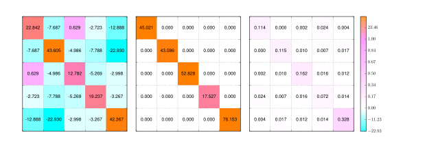
Here contains observed co-occurrences. can express that two different topics appear together. makes the link from those latent topics to words. An empirical matrix can fit the sample while violating properties the model needs, so the Rectified Anchor Word Algorithm adjusts it toward a valid structure before recovering the topics and their interactions.
The relationships between topics become data for another map
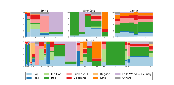
The third chapter refines the algorithm and then uses the learned topic-pair matrix as input to a second factorization. On the Songs dataset, the lower layer describes groups of tracks. The upper layer describes how those groups travel together. That makes each broad category traceable back to its constituent subtopics. Two systems can have the same number of broad labels while giving the listener different routes to the underlying songs.
A collection-level map leaves one document to explain
Knowing that two topics tend to appear together in the collection can help when a document uses few distinctive words. Prior-Aware Dual Decomposition, or PADD, uses that collection-level information while estimating a document’s own mix. The fourth chapter separates learning the topics from inferring which ones appear in an individual case. This lets the system use the already learned relationships without repeating corpus-wide estimation for every document.
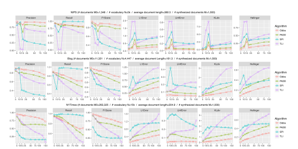
The table extracts unseen-document F1 values from Table 4.1. The comparison asks whether the estimated active topics agree with the compositions obtained by Gibbs sampling under the study’s setup. It is an agreement test against a model reference.
| Collection | Thresholded Linear Inverse (TLI) | SPI | PADD |
|---|---|---|---|
| NIPS | 0.536 | 0.307 | 0.744 |
| Blog | 0.527 | 0.289 | 0.715 |
| New York Times | 0.427 | 0.281 | 0.668 |
The dissertation brings three jobs into one sequence: obtain usable statistics, interpret relations across the collection, then apply them to one item. A very large vocabulary makes the first job costly because the matrix has room for every pair. The dissertation treats large-vocabulary compression as a separate line of work, which matters when taking the method from the test collections to a much larger archive.
Questions & Answers
The opening answers are simulated author responses based on the dissertation.
Q: What does an anchor word buy you?
A: In the model, an anchor occurs only in its topic. Its co-occurrence profile can serve as a reference point, and profiles for words shared among topics can be expressed using those reference points. In a real collection, candidate anchors need empirical scrutiny.
Q: Why learn supertopics from subtopics?
A: The second level is built from relationships learned among the first-level topics. It gives readers a direct path between broad groups and specific topics, even when a separately fit broad model partitions the collection differently.
Q: Can the same score validate the topic map and the topics assigned to one document?
A: These are separate tasks. For the map, check whether meaningful groups persist across different anchor selections, topic counts, and embedding initializations. For one document, the thesis compares topic assignments with Gibbs-sampling estimates. That measures agreement with a modeling reference. Independent labels would answer a different question about how closely the document’s topics match a reader’s judgment.
Future Ideas
Keep an archive’s topic map interpretable as it grows
Build a research-library navigator that preserves approved topic names while flagging changes in their supporting terms and documents. Compare successive quarterly snapshots with a system that refits and renames topics each time. Ask librarians to track known subjects and identify newly emerging ones. Measure time to verify a change, stable labels that remain accurate, and new subjects missed by either approach. Track anchor drift explicitly using the rectified pipeline and a set of previously labeled documents.